ParamDomainDetection.m

Go to the documentation of this file.

namespace models{
namespace motoneuron{
namespace experiments{


/* (Autoinserted by mtoc++)
 * This source code has been filtered by the mtoc++ executable,
 * which generates code that can be processed by the doxygen documentation tool.
 *
 * On the other hand, it can neither be interpreted by MATLAB, nor can it be compiled with a C++ compiler.
 * Except for the comments, the function bodies of your M-file functions are untouched.
 * Consequently, the FILTER_SOURCE_FILES doxygen switch (default in our Doxyfile.template) will produce
 * attached source files that are highly readable by humans.
 *
 * Additionally, links in the doxygen generated documentation to the source code of functions and class members refer to
 * the correct locations in the source code browser.
 * However, the line numbers most likely do not correspond to the line numbers in the original MATLAB source files.
 */

function  ParamDomainDetection() {
MinHz = 10;
MaxHz = 60;
/*  Depending on sample simulations, an upper limit polynomial is computed.
 * Here, the fibre type and mean activation current along the 60Hz-contour
 * are used to fit a polynomial that yields  the maximum mean input current
 * for any fibre type. */

basedir = fileparts(mfilename(" fullpath "));

/*  m = models.motoneuron.Model;
 * m.T = 432; % [ms]
 * m.UseNoise = true;
 * 
 * m.System.Params(1).Range = [0 1];
 * m.System.Params(2).Range = [.5 9];
 * 
 * ns = 5000;
 * m.Sampler.Samples = ns;
 * m.Sampler.Seed = 1;
 * 
 * m.off1_createParamSamples;
 * 
 * %% Datagen
 * ct = zeros(1,ns);
 * Hz = -Inf(1,ns);
 * 
 * pi = ProcessIndicator('Assembling frequency data',ns,false);
 * % for k = 1 : ns
 * parfor k = 1 : ns
 *     [t,y,ct(k)] = m.simulate(m.Data.ParamSamples(:,k),1);%#ok
 *     
 *     % Finde anzahl peaks
 *     np = 0;
 *     sign = y(2,:) > 50;
 *     if any(sign)
 *         % Strategie: finde die indices der daten > 50, und stelle fest wie viele sprünge (abstand
 *         % >5 in diskreten zeiteinheiten) darin vorhanden sind.
 *         np = 1 + length(find(diff(find(sign)) > 5));
 *     end
 *     % Mittlere frequenz
 *     Hz(k) = (np/m.T)*1000; % [Hz]
 *     pi.step;%#ok
 * end
 * pi.stop;
 * m.save;
 * ps = m.Data.ParamSamples;
 * modeldir = m.Data.DataDirectory;
 * 
 * % Colormap
 * mHz = min(Hz);
 * MHz = max(Hz);
 * detail = linspace(mHz,MHz,1000);
 * ncol = length(detail);
 * r = zeros(ncol,1);
 * g = zeros(ncol,1);
 * b = zeros(ncol,1);
 * 
 * % Eff min to MinHz
 * [~,minpos] = min(abs(detail-MinHz));
 * toolow = 1:minpos;
 * g(toolow) = linspace(0,.5,length(toolow));
 * b(toolow) = linspace(1,0,length(toolow));
 * 
 * % MaxHz to eff max
 * [~,maxpos] = min(abs(detail-MaxHz));
 * toohigh = maxpos:ncol; 
 * r(toohigh) = linspace(.5,1,length(toohigh));
 * b(toohigh) = linspace(0,.1,length(toohigh));
 * 
 * % Intermediate
 * good = minpos:maxpos;
 * g(good) = .9; 
 * r(good) = linspace(.4,.9,length(good));
 * cmap = [r g b];
 * 
 * %% Compute upper limit polynomial
 * ft1 = 0:.005:1;
 * mc1 = .5:.05:9;
 * [ft,mc] = meshgrid(ft1,mc1);
 * iHz = griddata(ps(1,:),ps(2,:),Hz,ft,mc);
 * [i,j] = find(iHz > MaxHz);
 * [j,ftcolidx] = unique(j);
 * i = i(ftcolidx);
 * x_ft = ft1(j);
 * fx_mc = mc1(i);
 * upperlimit_poly = polyfit(x_ft,fx_mc,3);
 * 
 * save(fullfile(basedir,'paramdomaindetection_withnoise'), 'ct', 'modeldir', 'ps', 'Hz', 'cmap', 'MinHz', 'MaxHz','upperlimit_poly','x_ft','fx_mc');
 * save(models.motoneuron.Model.FILE_UPPERLIMITPOLY, 'upperlimit_poly'); */

/* % Plots */
load(fullfile(basedir," paramdomaindetection_withnoise "));

pm = PlotManager;
pm.LeaveOpen= true;
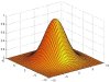
h = pm.nextPlot(" motoparamstudy "," Motoneuron firing rate in Hz for different parameters "," fibre_type "," mean_current_factor ");
tri = delaunay(ps(1,:),ps(2,:));
trisurf(tri,ps(1,:),ps(2,:),Hz," FaceColor "," interp "," EdgeColor "," interp ");
tricontour(gca, tri, ps" , Hz ",linspace(MinHz,MaxHz,5));
colormap(cmap);

h = pm.nextPlot(" upperlimitpoly "," Upper limit for mean current dependent on fibre type "," fibre_type "," mean_current_factor ");
plot(h,x_ft,fx_mc," b ",ft1,polyval(upperlimit_poly,ft1)," r ");

pm.done;
}
};
};
};